(this blog article is only available on the desktop version)


In this blog, I go over a classification run using mutliple classifiers for a 2-class problem involving bank data for which the goal is to predict a client making a term deposit (y/n) based on use of 20 input features and n=4119 records.
A citation for the data is S. Moro, P. Cortez and P. Rita. A Data-Driven Approach to Predict the Success of Bank Telemarketing. Decision Support Systems (2014), doi:10.1016/j.dss.2014.03.001, and they were downloaded from the UCI Machine Learning Repository. (the dataset employed is the "additional data," and not the larger "full" dataset).
The input features and their coding is as follows:
Input variables:
# bank client data:
1 - age (numeric)
2 - job : type of job (categorical: "admin.","blue-collar","entrepreneur","housemaid","management","retired","self-employed","services","student","technician","unemployed","unknown")
3 - marital : marital status (categorical: "divorced","married","single","unknown"; note: "divorced" means divorced or widowed)
4 - education (categorical: "basic.4y","basic.6y","basic.9y","high.school","illiterate","professional.course","university.degree","unknown")
5 - default: has credit in default? (categorical: "no","yes","unknown")
6 - housing: has housing loan? (categorical: "no","yes","unknown")
7 - loan: has personal loan? (categorical: "no","yes","unknown")
# related with the last contact of the current campaign:
8 - contact: contact communication type (categorical: "cellular","telephone")
9 - month: last contact month of year (categorical: "jan", "feb", "mar", ..., "nov", "dec")
10 - day_of_week: last contact day of the week (categorical: "mon","tue","wed","thu","fri")
11 - duration: last contact duration, in seconds (numeric). Important note: this attribute highly affects the output target (e.g., if duration=0 then y="no"). Yet, the duration is not known before a call is performed. Also, after the end of the call y is obviously known. Thus, this input should only be included for benchmark purposes and should be discarded if the intention is to have a realistic predictive model.
# other attributes:
12 - campaign: number of contacts performed during this campaign and for this client (numeric, includes last contact)
13 - pdays: number of days that passed by after the client was last contacted from a previous campaign (numeric; 999 means client was not previously contacted)
14 - previous: number of contacts performed before this campaign and for this client (numeric)
15 - poutcome: outcome of the previous marketing campaign (categorical: "failure","nonexistent","success")
# social and economic context attributes
16 - emp.var.rate: employment variation rate - quarterly indicator (numeric)
17 - cons.price.idx: consumer price index - monthly indicator (numeric)
18 - cons.conf.idx: consumer confidence index - monthly indicator (numeric)
19 - euribor3m: euribor 3 month rate - daily indicator (numeric)
20 - nr.employed: number of employees - quarterly indicator (numeric)
The output target is:
21 - has the client subscribed a term deposit? (binary: "1-yes","2-no")
Missing Attribute Values: There are several missing values in some categorical attributes, all coded with the "unknown" label. These missing values can be treated as a possible class label or using deletion or imputation techniques.
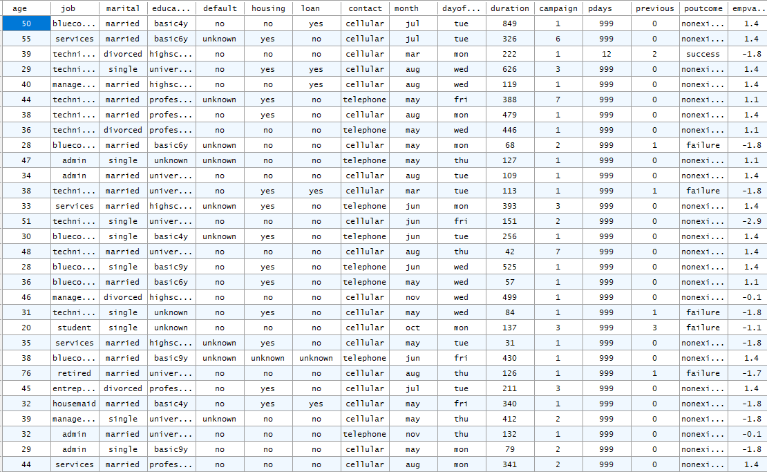
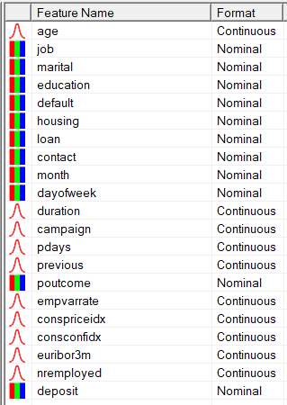
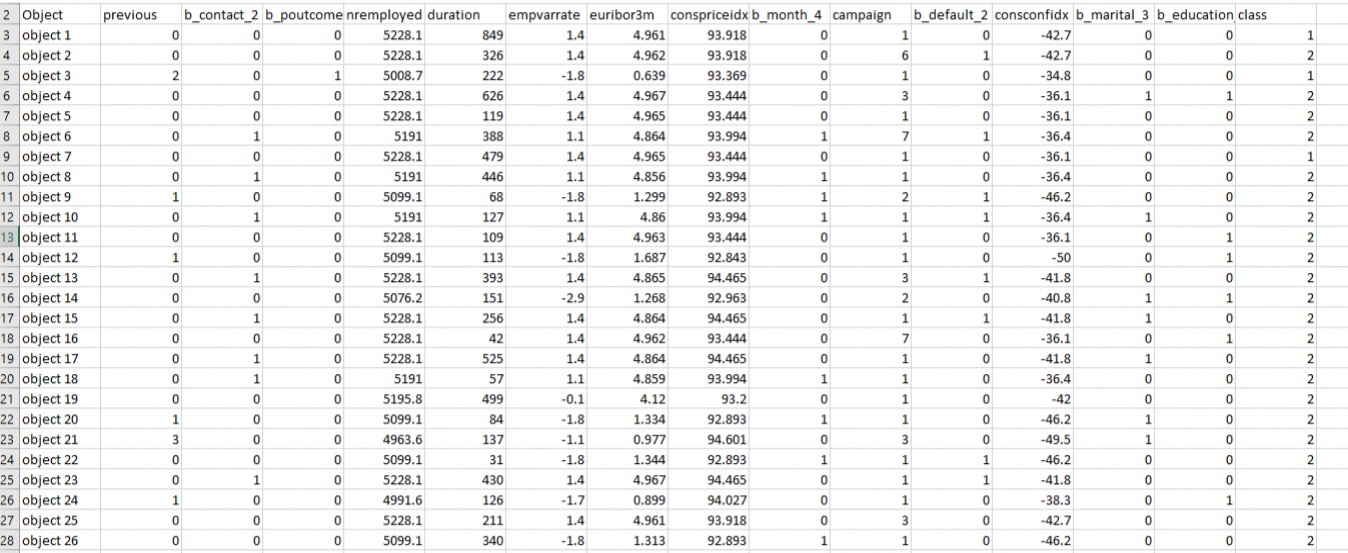
A problem for classification analysis regarding this dataset is that many input features are text-categorical. After import into Explorer, the results can be seen below:
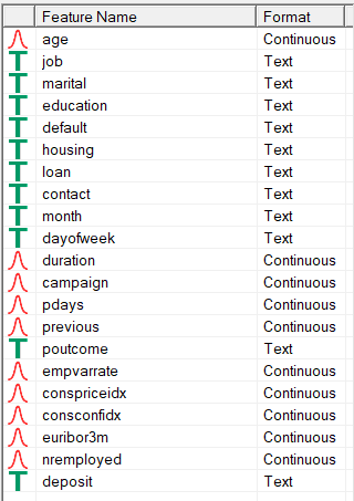
After import, the feature scale indicators (right side of screen) reveal the "T" for categorical text features:
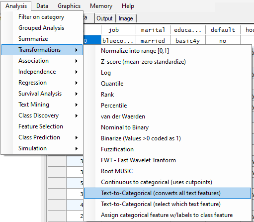
Fortunately, all of the text features can be rapidly transformed to numerical categorical features using the specific transformation to convert text to categorical:
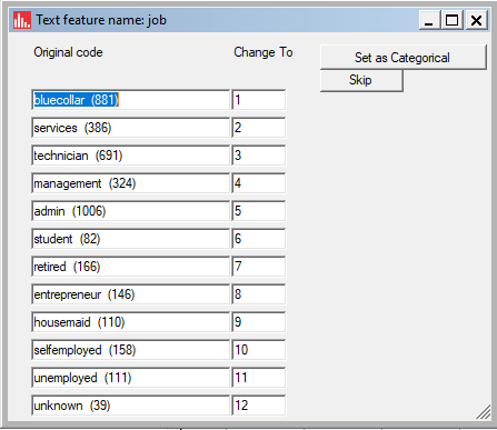
When running this transform, each text feature will present an option to "Set as categorical" or skip, so we specified "Set as categorical" for all the text features, one at a time.
Below is the list of categories automatically found for the "job" feature:
When done, the feature scale indicator will reflect that the text-category features were all transformed to categorical:
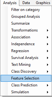
Next, because there are so many features, we ran Feature Selection:
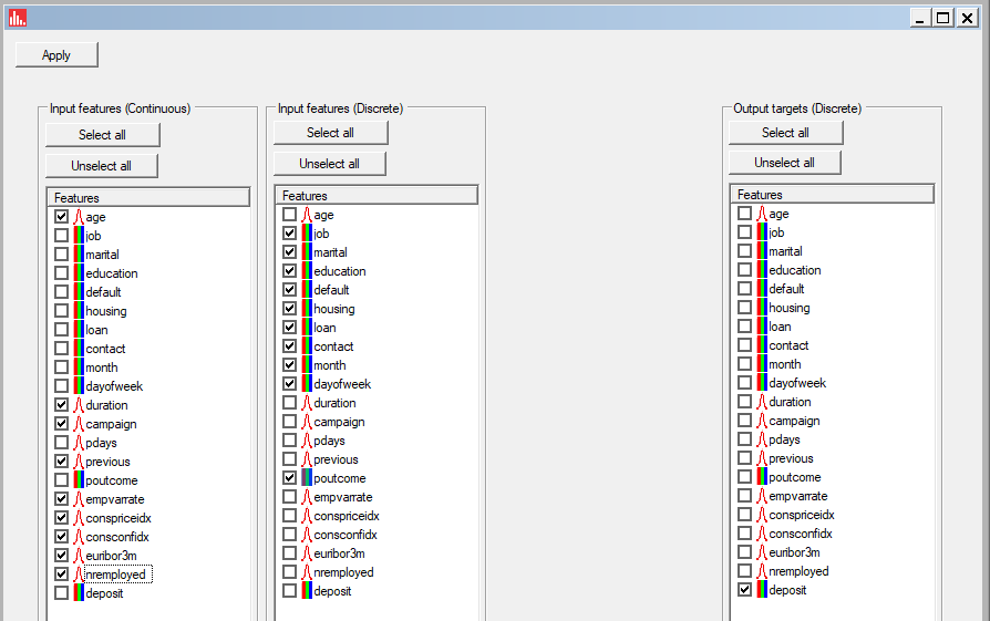
and then selected (specified) the continuous features as continuous, and categorical as discrete, along with specifying the class feature "deposit":
When discrete (categorical) features are input into Explorer, they are recoded to all possible binary features representing presence of (y/n) of each level of each categorical feature. The Mann-Whitney test was used to identify features which are significantly different across the two binary outcome classes. Since skewness and (min,max) of the continuous features were not evaluated (i.e., we don't know the skewness and whether there are outliers), the advantage of Mann-Whitney by default is that it won't be biased by outliers among continuous features. But as you know, if the assumptions for the t-test are met, use of Mann-Whitney will result in lower statistical power:
After the run, the following icons will be visible in the Treeview:
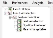
Click on the "Significant features" icon and you will notice the list of features whose values were significantly different across outcome class. Note that behind the scenes, Explorer recoded each level of the categorical factors into K binary (0,1) features representing each of the levels. This needed to be done since many of the categorical features in this dataset are nominal and not ordinal. It's inappropriate to directly input into any algorithm the actual nominal category levels (i.e., 1,2,3,...K) because for nominal features, the algorithm won't know the difference between 1 and K, since there is no mathematical distance between levels of nominal categorical features the same way there are for ordinally-ranked categorical features (e.g., 1-low, 2-medium, 3-high).
Therefore, it's faster to recode all categorical features into K binary features, since this is what any linear regression algorithm does for ordinally-ranked or nominal features anyhow. Thus, for Feature Selection, Explorer does this for every categorical feature, whether it's nominal or ordinal.
(the benefit of recoding category levels into all possible binary features, is that, irrespective of nominal or ordinal, certain levels of a factor may not be informative for contribution to the output, Thus, you don't want to take those levels into consideration -- so they are dropped from selection if not significant).
The new feature names of categorical features that are automatically recoded into binary are denoted by use of a "b_" in the prefix and "_k" (level) in the suffix. Several of these "binarized" features are listed below among features identified as significant:
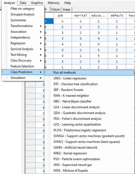
Now that the significant features have been identified, we will run Supervised class prediction using all methods:
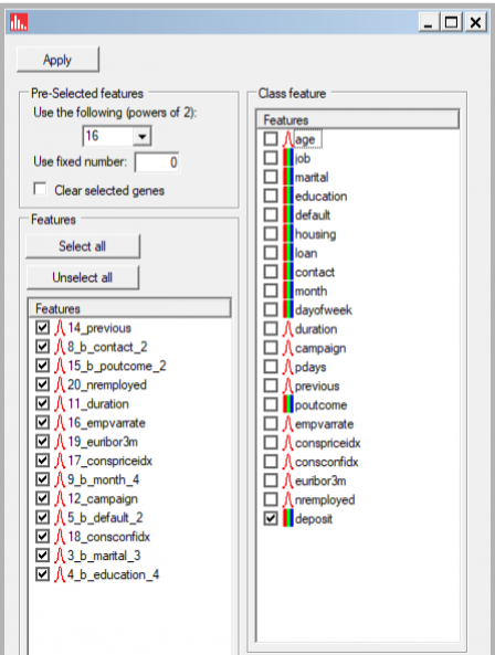
When selecting input features for class prediction, the list of features available for the run is auto-populated with features identified during feature selection (and this option can be turned off if desired):
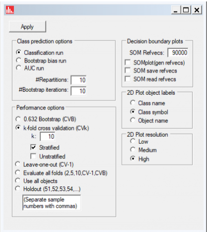
Accept the default values for cross-validation, and click on Apply:
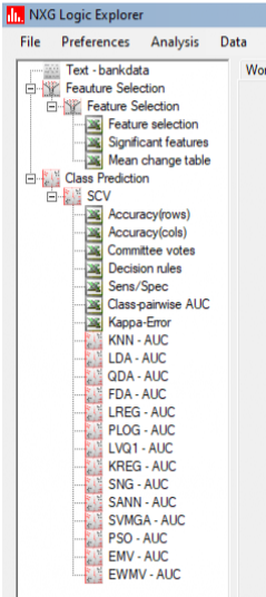
The list of output icons will become visible after the run has finished:
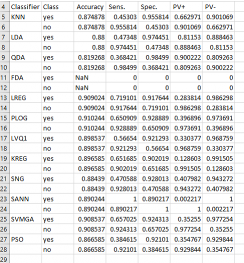
Clicking on sens/spec will show the class prediction accuracy for each classifier used as well and the class-specific sensitivity, specificity, PV+, and PV-. Note that the SANN classifier resulted in the greatest values of sensitivity and specificity.
A portion of the class-pairwise list of AUCs is shown below. Notice that the SANN classifier had an AUC of unity (one).
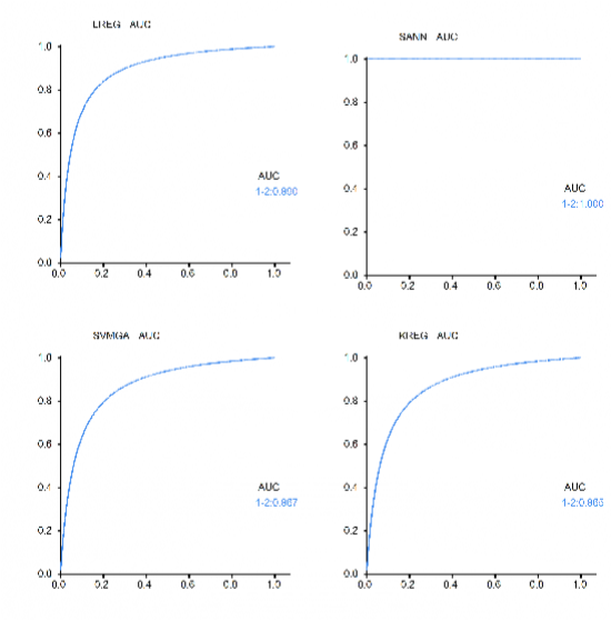
AUC plots for several of the classifiers are shown below. Not surprisingly, KREG performed very well. You can also see the AUC=1 for the SANN classifier, and linear regression performed about as well as the SVM:
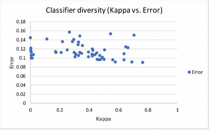
Using the diversity results for all possible combinations of classifiers used (i.e., "Kappa-Error" icon), we constructed a kappa vs. error plot: